
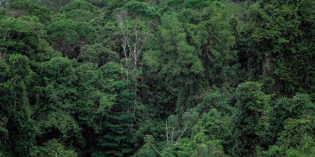
“How biodiverse is this place?” sounds like one question. It’s at least four, and each one gets a different tool. Biodiversity can be measured by what level of life you count, how far apart the sites are, which number you calculate, and how you collect the data in the first place. Most confusion comes from mixing those up.
This guide sorts the types of biodiversity measurement into those four groups, then works through a real calculation so you can see why a forest and a monoculture score so differently.
Contents
- The four types at a glance
- Type 1: Levels (genes, species, ecosystems)
- Type 2: Spatial scales (alpha, beta, gamma)
- Type 3: Metrics (richness, evenness, Shannon, Simpson)
- A worked example: forest vs. plantation
- Comparing sites: Jaccard and Sørensen
- Type 4: Data-collection methods
- What these numbers can’t tell you
- Which measure should you use?
The four types at a glance
| Type | What it answers | Typical tools | Use it when |
|---|---|---|---|
| Levels | Which part of life are we counting? | Genetic diversity, species diversity, ecosystem diversity | You’re framing the question or reading a policy document |
| Spatial scales | Is the variety within one site, between sites, or across a whole region? | Alpha, beta, gamma diversity | You’re comparing habitats or landscapes |
| Metrics | How do we turn the counts into a number? | Richness, evenness, Shannon, Simpson, Jaccard, Sørensen | You have species counts and need something comparable |
| Collection methods | How do we get the counts at all? | Transects, plots, camera traps, bioacoustics, eDNA, remote sensing | You’re designing a survey |
Think of it as a pipeline. You pick a level, choose a scale, collect data with a method, and summarize it with a metric.
Type 1: Levels (genes, species, ecosystems)
The Convention on Biological Diversity defines biodiversity as variability within species, between species and of ecosystems. Those are the three levels.
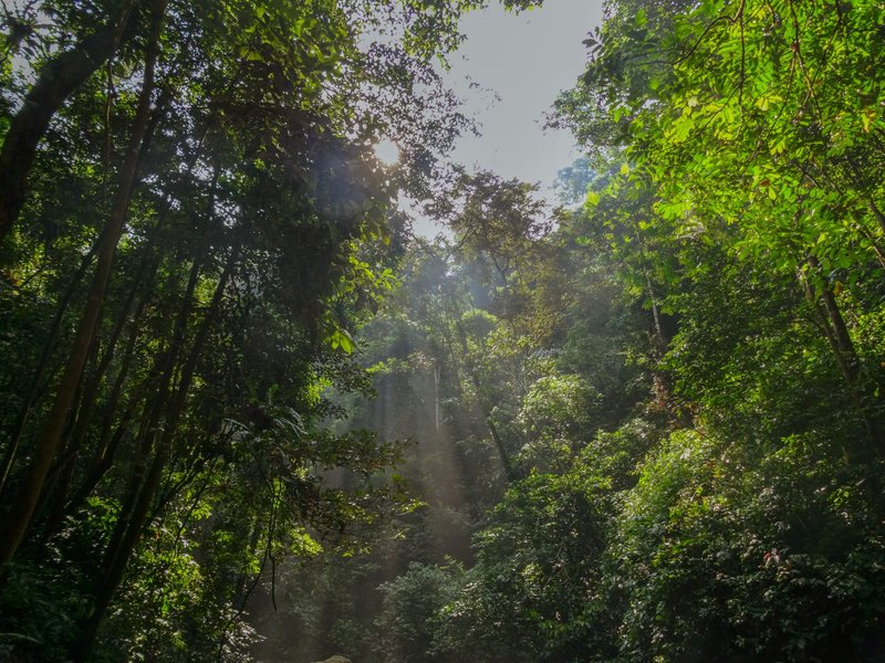
- Genetic diversity is variation in DNA within a species. A cheetah population with very little of it is vulnerable to a single disease. Measured with heterozygosity, allele counts or the number of distinct haplotypes.
- Species diversity is the variety of species in an area. This is what most people mean by “biodiversity,” and it’s where nearly all the classic indices live.
- Ecosystem diversity is the variety of habitats, communities and ecological processes: wetland, grassland, reef, forest. It’s usually measured by mapping habitat types and their areas.
Species diversity gets the most numbers because species are easy to define and count. Genetic and ecosystem diversity get less attention in the literature, but they matter just as much. A forest with ten tree species that are all clones of a few individuals is more fragile than the species count suggests.
Type 2: Spatial scales (alpha, beta, gamma)
Ecologist Robert Whittaker introduced this trio in 1960, and it’s still the standard way to say where diversity sits.
- Alpha diversity: the number or variety of species within a single site, such as one pond or one forest plot.
- Beta diversity: how much the species mix changes between sites. If two ponds share almost nothing, beta is high.
- Gamma diversity: the total diversity across the whole region, all sites combined.
The simplest relationship, Whittaker’s multiplicative version, is beta = gamma / mean alpha. A mountain range with ten identical-looking valleys has high alpha in each valley but low beta. A range where each valley hosts a different set of species has the same alpha but much higher beta and gamma.
This distinction changes conservation decisions. Protect one rich site and you save its alpha. Protect a network of different sites and you save the beta.
Type 3: Metrics (richness, evenness, Shannon, Simpson)
Once you have a species list with counts, you can calculate:
Species richness (S). The number of species. Easy to explain, easy to calculate, and blind to abundance. A site with 99 individuals of one species and 1 of another has the same richness as a site with 50 of each.
Species evenness. How equally individuals are spread among species. Pielou’s evenness is J = H / ln(S), where H is the Shannon index. It runs from near 0 (one species dominates) to 1 (perfectly equal).
Shannon index (H). Calculated as H = -Σ pᵢ ln(pᵢ), where pᵢ is the proportion of individuals belonging to species i. It combines richness and evenness, and it’s sensitive to rare species. Borrowed from information theory, it measures how hard it is to predict the species of a randomly picked individual.
Simpson index (D). Calculated as D = Σ pᵢ², the probability that two randomly picked individuals are the same species. Because a high D means low diversity, people usually report 1 − D (the Gini-Simpson index) or 1 / D (inverse Simpson). It is dominated by the common species, so rare ones barely move it.
That last point is the real difference between the two. Shannon gives rare species more weight. Simpson mostly asks who’s in charge.
Hill numbers unify all of this. They convert richness, Shannon and Simpson into “effective number of species” at different sensitivities to rarity (q = 0, 1 and 2). If you plan to publish, they’re worth learning. For everything else, Shannon and Simpson are enough.
A worked example: forest vs. plantation
Two 100-tree plots. Both contain five species.
| Species | Mixed forest (count) | Spruce plantation (count) |
|---|---|---|
| A | 20 | 96 |
| B | 20 | 1 |
| C | 20 | 1 |
| D | 20 | 1 |
| E | 20 | 1 |
Richness: 5 in both. By richness alone, they’re identical.
Mixed forest. Every proportion is 0.20.
- Shannon:
H = -5 × (0.2 × ln 0.2) = 5 × 0.2 × 1.609 = 1.609 - Simpson:
D = 5 × 0.2² = 0.20, so 1 − D = 0.80 and 1/D = 5.0 - Evenness:
J = 1.609 / ln 5 = 1.00
Spruce plantation. Proportions are 0.96 and four values of 0.01.
- Shannon:
H = -(0.96 × ln 0.96 + 4 × 0.01 × ln 0.01) = 0.039 + 0.184 = 0.223 - Simpson:
D = 0.96² + 4 × 0.01² = 0.9216 + 0.0004 = 0.922, so 1 − D = 0.078 and 1/D = 1.08 - Evenness:
J = 0.223 / 1.609 = 0.14
Same richness, wildly different stories. The forest behaves like five equally common species. The plantation behaves like barely more than one: its effective number of species is about 1.25 by Shannon (e^0.223) and 1.08 by Simpson.
Note how the two indices disagree on the plantation. Shannon is picking up the four rare species a little (1.25 vs. 1.08). Simpson largely ignores them. That’s the rarity-weighting difference from the previous section, in numbers.
Comparing sites: Jaccard and Sørensen
Alpha metrics describe one site. To quantify beta diversity between two, use a similarity index on presence/absence data.
Say Pond 1 has 10 species, Pond 2 has 8, and 4 species occur in both.
- Jaccard = shared ÷ total unique species =
4 / (10 + 8 − 4) = 4/14 = 0.29 - Sørensen =
2 × shared / (S₁ + S₂) = 8/18 = 0.44
Both range from 0 (nothing shared) to 1 (identical). Sørensen gives shared species double weight, so it always reads higher than Jaccard for the same data. Whittaker’s beta for these ponds: gamma is 14, mean alpha is 9, so beta is 14/9 ≈ 1.56. Values near 1 mean the sites are nearly the same. Values near 2 (for two sites) mean they share almost nothing.
Type 4: Data-collection methods
Metrics are only as good as the counts behind them. The method you pick decides which species you can possibly detect.
- Transects and quadrats. A transect is a line you walk and record along. A quadrat is a square plot you count inside. The classic approach for plants, intertidal organisms and anything that stays put.
- Point counts, mist nets and pitfall traps. Standard for birds (point counts, mist nets) and ground invertebrates (pitfall traps). Each biases toward the animals that behave in the way the trap expects.
- Camera traps. Motion-triggered cameras log mammals and ground birds that avoid people, around the clock, for weeks. They’re the best tool for shy, rare species.
- Bioacoustics. Autonomous recorders capture birds, frogs, bats and insects. Software such as BirdNET from Cornell’s Lab of Ornithology identifies species by call, so one recorder can cover hundreds of hours.
- Environmental DNA (eDNA). Animals shed skin, mucus and waste. Filter a liter of river water, sequence the DNA, and match it against reference libraries. It detects secretive fish and amphibians that nets miss, though it can’t tell you how many individuals there are, or whether the DNA drifted in from upstream.
- Remote sensing. Satellites and aircraft measure canopy height, vegetation type and habitat change across whole regions. NASA’s GEDI mission, run with the University of Maryland, uses a lidar on the International Space Station to map forest structure. That’s a proxy for habitat diversity, not a species count.
No single method catches everything, so serious surveys combine two or three.
Sampling also matters mathematically. A bigger sample always finds more species, so raw richness from a 10-hour survey and a 100-hour survey can’t be compared directly. Ecologists use rarefaction (resampling to equal effort) or estimators like Chao1 (which estimates how many species you missed) to level the field.
What these numbers can’t tell you
Every index flattens something.
- All species count equally. A critically endangered endemic and an invasive weed add the same +1 to richness. Neither Shannon nor Simpson knows which is on the IUCN Red List.
- Taxonomy isn’t ecology. Five closely related grasses and five species from five unrelated lineages score the same. Phylogenetic diversity (adding up evolutionary branch length) and functional diversity (the range of roles species play, such as pollinator, decomposer, predator) cover that gap.
- Presence isn’t persistence. A species detected once in a degraded fragment may be functionally gone. Zeta diversity extends beta to ask how many species are shared across three, four or more sites at once, which helps separate widespread species from rare, patchy ones.
- Scale changes the answer. A plot can score low in alpha and still be irreplaceable for gamma.
The honest takeaway is that diversity indices summarize a sample. They’re comparisons, not verdicts.
Which measure should you use?
Work from your question, not from the formula.
- Writing a policy or school paper? Frame it by the three levels: genetic, species, ecosystem.
- Comparing habitats or landscapes? Report alpha, beta and gamma. Add Jaccard or Sørensen for pairs of sites.
- Need one number for one site? Report richness and Shannon or Simpson. Richness alone hides dominance.
- Care about rare species? Use Shannon, or Hill numbers at q = 0 and 1.
- Care about which species dominate? Use inverse Simpson.
- Only have presence/absence data? Use richness, Jaccard and Sørensen. Shannon and Simpson need counts.
- Priorities are conservation value or ecosystem function? Add phylogenetic or functional diversity, since plain counts ignore both.
- Survey is hard to access or species are secretive? Use eDNA, camera traps or acoustic recorders in place of direct counts.
Whatever you choose, report the method and the sampling effort alongside the number. Of all the types of biodiversity measurement, the field method is the one most often left out, and it’s the one that decides whether two numbers can be compared at all.