In the 1780s Charles‑Augustin de Coulomb ran experiments that helped separate static hold from sliding resistance — the roots of modern friction theory. That distinction matters in everyday life: why does a stopped car grip the road better than a skidding one? Engineers and students often conflate static and sliding behavior and then design actuators, brakes, or bearings that fail or wear prematurely. This article lays out ten clear, practical differences so you can see how static and sliding friction differ at both the bench and in real systems.
Core Physical Differences
These three points cover the textbook distinctions you see in classrooms and labs: what stops motion, what resists motion once it starts, and how frictional force responds to applied loading.
1. Magnitude: μs is larger than μk
The coefficient of static friction μs is typically larger than the coefficient of kinetic friction μk, so you must usually push harder to start motion than to keep it going. Classical Coulomb–Amontons laws capture this: Fstatic ≤ μs·N, while during steady sliding Fkinetic ≈ μk·N.
Common ranges illustrate the point: rubber on dry concrete might have μs ≈ 1.0 and μk ≈ 0.8; steel‑on‑steel dry contacts often show μs about 0.6–0.8 and μk around 0.4–0.6. These numbers explain why heavy machinery needs a larger start torque and why a stuck vehicle often frees up once you get it moving.
Concrete example: a loaded shopping cart requires a noticeable extra shove to overcome μs, then much less steady force to coast—exactly the μs>μk effect Coulomb and Amontons characterized in the 1780s and early tribology work.
2. Threshold vs continuous resistance
Static friction provides a threshold: it adaptively cancels applied tangential forces up to a maximum value μs·N and prevents motion. Once that threshold is exceeded, sliding begins and kinetic friction provides a typically lower, continuous opposing force ≈ μk·N.
Mathematically, the sticking condition is Fapplied ≤ Fmax = μs·N, and during sliding F ≈ μk·N. That simple inequality captures why doorstops, clamps, and angle‑of‑repose tests use the threshold, while conveyor belts and sliding bearings contend with steady drag.
Concrete example: a stuck drawer takes an extra shove to start moving; once it slides the force drops to a roughly constant level. A simple tilt or incline test (tanθ = μs) demonstrates the threshold behavior in the lab.
3. Adaptive direction and magnitude vs fixed opposition
Static friction is adaptive: both its magnitude (up to μs·N) and its direction change to exactly oppose the resultant of applied forces while the contact remains stationary. Kinetic friction, by contrast, acts in a fixed sense—opposing the direction of sliding with a roughly constant magnitude.
Imagine gradually increasing a horizontal push on a block. Static friction grows to match the push, up to μs·N; when the block yields, kinetic friction steps in and resists motion in the opposite direction at about μk·N. That adaptivity is why clamps and brake pads can hold parts in position without continuous control effort.
Concrete example: a bicycle parked on a slope remains at rest because static friction balances gravity until the angle exceeds μs·N; once slipping begins, kinetic friction governs descent and is less effective at stopping motion.
Microscopic and Material Behavior

Friction comes from tiny contact spots (asperities) and material response; static and kinetic regimes differ in how those microcontacts form, deform, and dissipate energy during stick and slip.
4. Contact mechanics: asperities and real contact area
The apparent contact area between bodies usually overstates the true load‑bearing area. Real contact area is a patchwork of asperity contacts that grows with normal load and depends on hardness or elastic modulus.
Contact mechanics theory (Hertzian and subsequent models) shows real area ∝ Normal force/Hardness for many nonconforming contacts. That explains numeric behavior: increasing inflation or adding tread can alter the effective contact patch and change μ values for tires, for example.
Concrete examples: polished metal makes few large contact spots and may show different μs/μk than rough sandpaper, while rubber on asphalt uses many small contacts whose real area and viscoelastic response shape grip under both static and sliding conditions.
5. Energy dissipation: heat, wear, and irreversible processes
During sliding, mechanical work converts into heat, plastic deformation, and wear particles—processes that don’t occur while two surfaces merely sit together. Static contact stores elastic energy in asperities until slip releases it abruptly.
Quantified examples illustrate scale: repeated braking can raise rotor surface temperatures by hundreds of degrees Celsius in seconds, altering μk and producing wear. Tribology studies and ASTM test methods document wear rates and the thermal sensitivity of friction materials.
Practical consequences include brake fade, clutch glazing, and the need for lubricants or dry coatings (graphene or MoS2) to reduce heat generation and wear in sliding contacts.
Dynamics, Velocity Dependence, and Instabilities

Friction during motion is not always constant: history, speed, and contact evolution make kinetic friction richer and more variable than the static threshold.
6. Velocity dependence and the Stribeck effect
Kinetic friction often depends on sliding speed. In lubricated contacts the Stribeck curve shows μk decreasing with increasing speed in a boundary‑to‑mixed regime, with the low‑speed region sometimes occurring below a few millimetres per second for thin films.
This behavior matters for bearings and brakes: initial slow slide feels different than high‑speed skidding, and designers tune surface roughness, lubricants, and clearance to place operating speeds in favorable parts of the Stribeck curve.
Concrete example: a brake pad exhibits higher friction at low relative sliding speeds and different frictional heating at high speeds, which engineers model when designing brake fade resistance.
7. Stick-slip and hysteresis during transition
Stick‑slip arises when the system alternates between sticking (governed by μs) and slipping (μk), typically when μs>μk and loading or drive stiffness creates intermittent release. The result is oscillation, noise, and extra wear.
Applications span from violin bows and drilling to precision stages and earthquake faults. Frequency and amplitude depend on system stiffness, mass, and the μs−μk gap; lubrication or damping often suppresses the instability.
Concrete example: a squeaky hinge is a low‑energy stick‑slip device—add oil or grease to reduce μs or increase damping and the squeak and wear disappear.
8. Modeling approaches: threshold laws vs rate-and-state and empirical laws
Simple engineering often uses Coulomb’s threshold model for static friction and a constant μk for sliding. Advanced problems use empirical velocity‑dependent laws or rate‑and‑state formulations from seismology and modern tribology to capture time, speed, and contact history effects.
Rate‑and‑state laws include internal state variables for contact age and real area, enabling prediction of phenomena like velocity‑weakening or strengthening that simple Coulomb models miss. Control engineers compensate stiction with deadband algorithms or add preload to avoid the uncertain static regime.
Concrete example: precision robotic servomotors use controller deadband compensation to overcome static friction, while tire and vehicle dynamic models include speed‑dependent μk curves for traction prediction.
Measurement, Engineering, and Real-world Implications

Clear testing and conservative design choices depend on recognizing the differences between static and kinetic friction: you use μs to size holds and actuators, and μk to predict sliding losses, wear, and heat.
9. Measurement techniques: tilt-table, sled tests, and standards
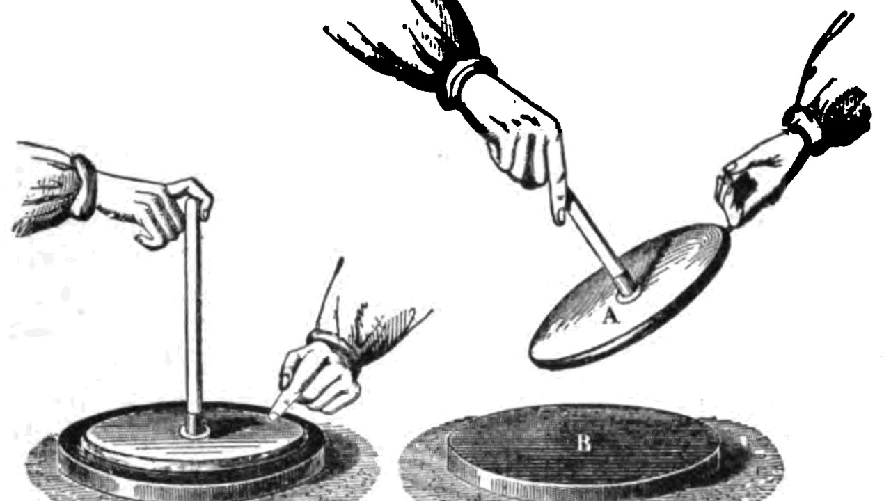
Common lab methods separate regimes: tilt or angle‑of‑repose tests give μs via tanθ = μs, while sled or tribometer runs produce μk as an average sliding resistance under controlled normal load and speed.
Standards organizations such as ASTM publish protocols for repeatable friction and wear testing. Repeatability matters—surface prep, humidity, and test speed shift measured values. Example: μs = 0.5 corresponds to a tilt angle of about 26.6° (tan⁻¹0.5 ≈ 26.6°).
Real-world applications include brake and tire labs that run controlled sled tests for traction, and material qualification where manufacturers track μk under representative sliding speeds.
10. Design and safety implications: margins, lubrication, and control
The μs>μk gap directly informs safety margins and component sizing: designers take the larger static coefficient when preventing motion and use μk plus wear/thermal allowances for sliding predictions. A common rule of thumb is to include a 20–30% margin above expected μs‑limited loads to account for variability and aging.
Engineers apply lubrication, coatings (graphene, PTFE), or surface texturing to reduce μk and wear, and they tune control systems to overcome stiction without exciting stick‑slip. Automotive ABS uses rapid modulation to avoid sustained sliding and exploit higher static/dynamic traction behavior at the tire‑road interface.
Concrete examples: tire makers publish dry/wet μ values for traction; fasteners get anti‑seize to avoid galling; clutch designers manage controlled slip using known μk and thermal limits.
Summary
- Static friction provides a selectable hold up to μs·N; kinetic friction gives a lower, continuous opposing force during sliding.
- Microscopic contact area and asperity deformation explain why μs usually exceeds μk and why heat and wear accompany sliding.
- Friction during motion depends on speed and history (Stribeck curves, stick‑slip), so kinetic behavior often requires richer models than a simple threshold law.
- Engineers measure μs with tilt tests and μk with sled/tribometer runs, and they design with the larger static coefficient for hold cases while addressing μk for sliding losses and wear.
- Check material‑specific μ values (tire vs pavement, brake pad data) or ASTM/tribology references when start‑stop performance or sliding losses are critical; consider lubrication or surface treatment to control μk.