Euclid’s Elements (c. 300 BCE) codified geometric construction and proof, shaping how generations learned to reason about space and proportion.
That same impulse to externalize thought — to write, draw, and test ideas — runs from ancient manuscripts through classroom blackboards to laptop-based notebooks. Tools help mathematicians think, compute, and communicate; they shorten the path from intuition to rigorous argument.
From pencil-and-paper proofs to Wolfram Mathematica and MATLAB, understanding these ten tools used in mathematics reveals how different instruments serve distinct purposes: foundational, computational, visualization, and applied. The list that follows mixes low-tech items like compass-and-straightedge and the TI-84 Plus (introduced 2004) with high-tech systems such as Mathematica and Python, showing the continuity of practice across centuries.
Foundational Tools: Thinking with Hands and Head
Low-tech tools remain central because they let us externalize reasoning, test hypotheses quickly, and build intuition before formalizing results. A sketch on paper often exposes a hidden symmetry or counterexample faster than hours of symbolic manipulation.
These instruments also enforce precision: drawing a perpendicular with a straightedge and compass or writing a careful proof encourages habits that carry into formal mathematics. That pedagogical value explains why Euclid’s Elements (c. 300 BCE) and high-school geometry classes still share the same constructive spirit.
Finally, foundational tools are cheap, portable, and immediate, which makes them indispensable in classrooms and research alike. Whether a student uses a compass to bisect an angle or a researcher sketches a homotopy diagram, the hand-and-head workflow remains the bedrock of discovery.
1. Paper and Pencil
Paper and pencil are the oldest and still most versatile tools for exploring ideas. From Euclid (c. 300 BCE) and Archimedes to modern research notebooks, handwriting and sketching let you try approaches that would be cumbersome to encode immediately.
In practice, mathematicians use paper for proof scribbles in topology, rough calculations before coding a simulation, and exam scratchwork. A short handwritten derivation often becomes the backbone of a later LaTeX write-up or a reproducible notebook.
Good habits speed work: sketch diagrams, label axes, number steps, and keep dated, organized notes so an old idea can be retrieved and refined.
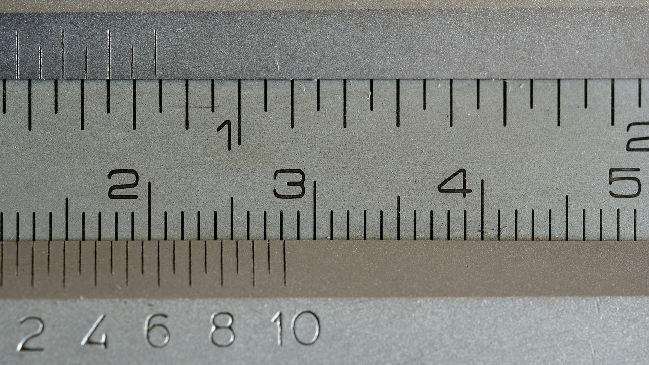
2. Ruler and Compass (Straightedge and Compass)
Ruler-and-compass constructions formalize geometric reasoning by restricting operations to drawing straight lines and circles, which teaches both technique and the limits of construction.
Classical results—bisecting angles, constructing perpendiculars, and making regular polygons—are practiced with these tools in classrooms and underpin proofs in Euclidean geometry. They also clarify what cannot be done: classical impossibilities like angle trisection or squaring the circle illustrate intrinsic constraints.
Concrete exercises, such as constructing a perpendicular bisector or the regular pentagon, reinforce precision and help students develop geometric intuition.
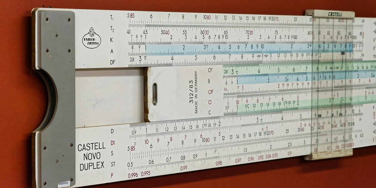
3. Scientific and Graphing Calculators
Calculators speed numeric work and are standard in teaching and applied mathematics. The TI-84 Plus, introduced in 2004, is one familiar example, while HP scientific models remain common in engineering settings.
These devices let students plot functions, solve equations numerically, and perform iterative computations during labs. For instance, a student can quickly test root-finding approaches on a quadratic, or an engineer can check a hand-derived estimate before running a full simulation.
Graphing calculators are portable exploration tools—handy for quick checks, classroom demonstrations, and examinations where computers are restricted.
Analytical & Computational Tools: From Symbolic Algebra to Code
Symbolic solvers, numerical packages, and programming languages let mathematicians scale work, test conjectures computationally, and make experiments reproducible. Each category serves different needs: symbolic systems manipulate expressions exactly, numerical environments handle large-scale approximations, and programming languages automate workflows.
Historical milestones mark this evolution: Wolfram Mathematica first appeared in 1988, MATLAB was commercialized in 1984, Python debuted in 1991, and R followed in 1993. These platforms moved computation from bespoke code into shared ecosystems.
Choosing between symbolic, numeric, or programmatic tools depends on the task: proving an identity favors a computer algebra system, solving a discretized PDE needs a numerical environment, and building a reproducible pipeline calls for a programming language and version control.
4. Symbolic Algebra Systems
Symbolic systems perform algebraic manipulation, exact simplification, and symbolic integration or differentiation, making them ideal for closed-form work. Wolfram Mathematica (1988) and Maple are long-standing commercial options; SymPy provides an open-source alternative within Python.
Researchers use these systems to derive closed-form solutions, simplify lengthy expressions, and verify identities that would be tedious by hand. For example, a symbolic integrator can produce an exact antiderivative, or a CAS can factor a large polynomial to expose structure.
Licensing matters: commercial systems offer polished features and support, while open-source libraries make it easier to embed symbolic work in reproducible Python workflows.
5. Numerical Computing Environments
Environments such as MATLAB (commercial), NumPy/SciPy in Python, and GNU Octave handle large numerical datasets, linear algebra, and numerical solvers. MATLAB established itself in engineering in the 1980s, while Python’s scientific stack gained mass adoption through the 2010s.
Typical applications include eigenvalue problems, discretized PDE solvers, and data-analysis pipelines. For instance, one might solve a finite-difference discretization of a heat equation in MATLAB or perform large matrix factorizations with NumPy.
These tools balance prototyping speed and scalability; high-level interfaces let you test ideas quickly while compiled libraries under the hood deliver performance.
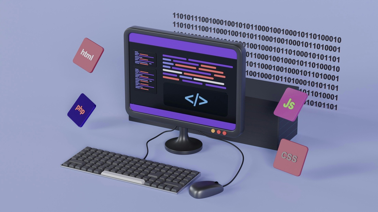
6. Programming Languages for Mathematical Work
Languages like Python (1991), R (1993), and Julia (2012) let mathematicians automate experiments, implement algorithms, and build reproducible analysis pipelines. Python offers breadth through libraries such as NumPy, SciPy, and SymPy; Julia aims for high-performance numerical computing.
Common tasks include Monte Carlo simulations, building custom solvers, and creating reusable research code. For example, a Monte Carlo integration in Python can be prototyped quickly, then ported to Julia if speed becomes critical.
When selecting a language, weigh ease of use and ecosystem against raw performance—often a mixed approach (Python for orchestration, compiled kernels for heavy lifting) is best.
Visualization & Communication Tools: Making Ideas Visible

Visualization and clear presentation are essential for spotting mistakes, conveying proofs, and teaching concepts. Interactive graphs and publication-quality typesetting help readers see structure and follow arguments.
Notable tools include GeoGebra (2001) and Desmos (2011) for classroom interactivity, and TeX (1978) with LaTeX popularized in the 1980s for typesetting. Plotting libraries like Matplotlib and ggplot2 produce figures suitable for journals and talks.
Well-crafted visuals reduce cognitive load: a phase-plane plot or a slider-driven demo can reveal parameter dependence faster than pages of algebra.
7. Graphing and Visualization Software
Visualization software turns abstract formulas into visual intuition. GeoGebra (2001) and Desmos (2011) are classroom-friendly, while Matplotlib, Plotly, and specialized tools serve research-grade figures.
Use interactive sliders to show how parameters affect roots, generate phase-plane plots to study ODE behavior, or produce heatmaps for numerical solutions of PDEs. These visuals support exploration and make it easier to spot anomalies.
Interactive demos engage students and help researchers sanity-check models before committing to heavy computation.
8. Typesetting and Documentation (LaTeX and TeX)
TeX, developed by Donald Knuth in 1978, and LaTeX (widely used from the 1980s) produce consistent, professional mathematical notation for papers, books, and lecture notes. They remain the standard for publication-quality documents.
LaTeX integrates with tools like Overleaf for collaborative editing and with Jupyter or knitr to mix code, figures, and mathematics for reproducible research. Bibliographies and cross-references are handled cleanly via BibTeX or newer packages.
For newcomers, web-based editors and templates lower the entry barrier so authors can focus on content instead of configuration.
Applied & Specialized Tools: Statistics, Modeling, and Simulation
When mathematics meets data and physical systems, specialists turn to statistical packages, modeling platforms, and domain-specific toolchains. These tools bridge theory and experiment, making models testable, validated, and usable in industry.
Examples include R (first released 1993) for statistical analysis, COMSOL (company founded 1986) for multiphysics simulation, and Simulink (MathWorks) for control-system prototyping. Such platforms are used across pharmaceuticals, engineering, and the social sciences.
Applied tools emphasize reproducibility and validation: simulations must be compared to data, and statistical models must survive robustness checks before being trusted in decision-making.
9. Statistical and Data Analysis Software
Statistics tools let mathematicians and analysts handle data, fit models, and test hypotheses. R, first released in 1993, along with commercial packages like SPSS and SAS, power analyses in many industries.
Practical uses include running regressions, performing bootstraps, and conducting permutation tests. Clinical trials often rely on validated statistical code in SAS, while economists commonly use R or Stata for panel regressions.
Open-source ecosystems encourage transparency and reproducibility, which matters in regulated settings like pharmaceuticals or government research.
10. Mathematical Modeling & Simulation Tools
Simulation platforms let mathematicians test models against realistic scenarios. COMSOL (company founded 1986) and Simulink (MathWorks) are examples used to model heat transfer, structural dynamics, and control systems.
Applications range from agent-based epidemiological models to finite-element simulations for engineering. A researcher might simulate a PDE in COMSOL, prototype a controller in Simulink, or run an agent-based model to explore disease spread.
Trade-offs include validation effort and computational cost: realistic simulations can be expensive, so model reduction and sensitivity analysis are routine parts of the workflow.
Summary
- Paper-and-pencil methods remain invaluable for quick insight, while digital tools scale, automate, and formalize those ideas.
- Symbolic and numeric systems serve different roles: one gives exact manipulation, the other tackles large-scale approximation and data.
- Visualization and clear typesetting accelerate communication and error checking; interactive graphers like GeoGebra or Desmos are great places to start.
- Try one new tool this week — open a short NumPy example, experiment with a GeoGebra demo, or load a LaTeX template on Overleaf — to sharpen your workflow.