From GPS routing to social-network analysis, the algorithms that work on graphs shape how systems model relationships and find solutions across domains like mapping, recommendation, and bioinformatics. A practical sense of what each method does and when to use it saves time and avoids costly mistakes.
There are 48 Graph Algorithms, ranging from A* to the Weisfeiler–Lehman test; for each algorithm the data are organized under Problem solved, Time complexity, Common use cases — you’ll find below.
How do I choose the right graph algorithm for my problem?
Start by clarifying the graph type (directed vs. undirected, weighted vs. unweighted), the question you need answered (shortest path, connectivity, matching, isomorphism, etc.), and constraints like graph size or real-time needs; then use the Problem solved and Time complexity columns below to filter candidates and the Common use cases to match practical examples.
Can these algorithms handle very large, real-world graphs?
Many can, but scalability depends on complexity and implementation: prefer linear or near-linear methods, streaming/approximate approaches, or parallel implementations for massive graphs; consult the Time complexity and Common use cases entries below to spot algorithms proven in large-scale scenarios.
Graph Algorithms
| Algorithm | Problem solved | Time complexity | Common use cases |
|---|---|---|---|
| BFS | Find shortest unweighted paths from a source | O(V+E) | Shortest paths in unweighted graphs, level-order traversal |
| DFS | Explore all reachable nodes and discover structure | O(V+E) | Topological order, cycle detection, maze solving |
| Bidirectional BFS | Shortest path between two nodes in unweighted graphs | O(V+E) worst-case, often faster | Route finding in large networks, puzzle solvers |
| Dijkstra | Shortest paths from a source with nonnegative weights | O((V+E) log V) | Routing, maps, network latency, pathfinding |
| Bellman–Ford | Shortest paths with possibly negative edges; detects negative cycles | O(VE) | Currency arbitrage, graphs with negative weights |
| A* | Heuristic-guided shortest path with nonnegative weights | O((V+E) log V) typical | Game AI, maps, robotics path planning |
| Johnson | All-pairs shortest paths for sparse graphs | O(VE + V^2 log V) | All‑pairs on sparse graphs, reuse single‑source solvers |
| Floyd–Warshall | All‑pairs shortest paths (dense graphs) | O(V^3) | Small dense graphs, transitive closure, dynamic programming |
| Shortest paths in DAG | Single-source shortest paths in directed acyclic graphs | O(V+E) | Scheduling, DP on DAGs, critical path |
| Multi-source BFS | Distances from multiple starting nodes in unweighted graphs | O(V+E) | Nearest facility queries, multi-source labeling |
| Kruskal | Minimum spanning tree via edge-sorting | O(E log E)≈O(E log V) | Network design, clustering, MST proofs |
| Prim | Minimum spanning tree via greedy growth from a node | O(E + V log V) | Network infrastructure, MST maintenance |
| Borůvka | Parallel-friendly MST via component contraction | O(E log V) | Parallel/distributed MST, initial merging phases |
| Ford–Fulkerson | Compute maximum flow using augmenting paths | O(E · f) where f is max flow | Network throughput, bipartite matching (via flow) |
| Edmonds–Karp | Max flow with BFS shortest augmenting paths | O(VE^2) | Network flow, routing, matching |
| Dinic | Max flow using layered graphs and blocking flows | O(V^2E) worst-case, faster in practice | High-performance flow, bipartite matching |
| Push–relabel | Max flow via local pushes and relabels | O(V^3) worst-case, often faster | High‑performance max flow, dense graphs |
| Stoer–Wagner | Global minimum cut for undirected graphs | O(VE + V^2 log V) | Network reliability, partitioning |
| Karger’s contraction | minimum cut via randomized edge contractions | O(E log^2 V) randomized expected | Approximate global min‑cut, randomized algorithms |
| Hopcroft–Karp | Maximum matching in bipartite graphs | O(√V E) | Job assignment, resource allocation |
| Blossom (Edmonds) | Maximum matching in general graphs | O(V^3) | General matching, scheduling, chemistry graph problems |
| Hungarian (Kuhn–Munkres) | Minimum-cost perfect matching in bipartite graphs | O(n^3) | Assignment problems, scheduling, resource matching |
| Kosaraju | Strongly connected components in directed graphs | O(V+E) | SCC detection, condensation, program analysis |
| Tarjan SCC | Strongly connected components using one DFS | O(V+E) | SCCs, compiler analysis, graph condensation |
| Connected components (BFS/DFS) | Partition nodes into connected components | O(V+E) | Component labeling, image segmentation, clustering |
| Bridges and articulation points | Find edges/nodes whose removal disconnects graph | O(V+E) | Network vulnerability, reliability analysis |
| Biconnected components | Decompose graph into biconnected subgraphs | O(V+E) | Network resilience, block‑cut trees, planarity checks |
| Topological sort (Kahn) | Linear ordering of DAG nodes respecting edges | O(V+E) | Scheduling, build systems, course prerequisites |
| Brandes (betweenness) | Compute betweenness centrality for all nodes | O(VE) unweighted typical | Network analysis, influencer detection |
| PageRank | Node importance via random-walk stationary distribution | O(I·(V+E)) per iteration | Web ranking, influence scoring, recommendation weighting |
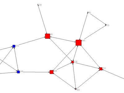
| Spectral clustering | Graph partitioning using Laplacian eigenvectors | O(V^3) (eigen decomposition) | Community detection, image segmentation |
| Louvain method | Fast modularity-based community detection | O(V log V) typical | Large-network community detection, social graphs |
| Girvan–Newman | Community detection via iterative edge removal | O(VE^2) expensive | Understanding community structure, exploratory analysis |
| Label propagation | Fast, local community detection by label diffusion | O(E) per iteration | Large graphs, streaming-like community detection |
| Node2vec | Learn node embeddings via biased random walks | O(number_of_walks·walk_length) per epoch | Representation learning, link prediction, classification |
| DeepWalk | Node embeddings from uniform random walks and Skip‑Gram | O(number_of_walks·walk_length) per epoch | Unsupervised embeddings, clustering, link prediction |
| LINE | Large-scale network embeddings preserving first- and second-order proximities | O(E) per epoch | Scalable embeddings, social networks, recommendation |
| Weisfeiler–Lehman test | Graph isomorphism heuristic and feature extractor | O(h·(V+E)) where h iterations | Graph kernels, isomorphism testing, embeddings |
| K‑core decomposition | Peel graph into cores by degree threshold | O(V+E) | Network robustness, cohesive subgraph analysis |
| Chinese Postman (Route inspection) | Shortest closed walk visiting every edge at least once | Polynomial; matching step O(V^3) | Logistics, street routing, maintenance scheduling |
| Christofides’ algorithm | Approximate metric TSP within 1.5× optimum | O(V^3) | Route planning, vehicle routing approximations |
| VF2 | Subgraph isomorphism and pattern matching | Exponential worst-case | Chemical structure search, pattern matching |
| Karp’s minimum mean cycle | Minimum mean-weight cycle in directed graphs | O(VE) | Negative-cycle analysis, periodic scheduling |
| Graph coloring (DSATUR) | Color vertices with minimum colors heuristically | NP-hard; DSATUR O(V^2) | Register allocation, scheduling, frequency assignment |
| Subgraph centrality (spectral) | Node importance via closed walks and eigenvalues | O(V^3) (eigen computations) | Network role analysis, motifs, influence |
| Maximum spanning forest | Maximize total weight without cycles across components | O(E log V) | Maximum reliability subnetwork, diversity spanning trees |
| Minimum feedback edge set | Remove edges to eliminate cycles (minimization) | NP-hard; approximations polynomial | Deadlock resolution, circuit design, DAG conversion |
| K‑means on graph embeddings | Cluster nodes after embedding into Euclidean space | O(k·V·t) per run | Community discovery after embedding, segmentation |
Images and Descriptions
BFS
Breadth‑first search explores a graph layer by layer from a start node to find shortest unweighted paths, discover components, and compute distances. Use when edges are unweighted; it’s simple, linear-time, and good for reachability and layering tasks.

DFS
Depth‑first search dives deep into neighbors recursively to explore structure and detect cycles, components, or back edges. It’s memory‑efficient, useful for component discovery, topological sorting, and many graph decompositions requiring discovery/finish times.
Bidirectional BFS
Runs two simultaneous BFS searches from source and target and meets in the middle to drastically reduce explored nodes on many graphs. Best for single-pair queries on large unweighted graphs; worst-case still linear.
Dijkstra
Efficient single‑source algorithm for graphs with nonnegative edge weights using a priority queue. Provides exact shortest paths; choose when weights are ≥0. Complexity depends on heap; not suitable for negative edges.
Bellman–Ford
Bellman–Ford relaxes edges repeatedly to compute single‑source shortest paths allowing negative edges and detects negative cycles. Simpler but slower than Dijkstra; use when negative weights exist or cycle detection matters.
A*
A* augments Dijkstra with an admissible heuristic to guide search toward the goal, often reducing explored nodes dramatically. Use when you can supply a good heuristic estimating remaining distance.
Johnson
Johnson’s algorithm reweights edges with Bellman‑Ford, then runs Dijkstra from each node. Efficient for sparse graphs where Floyd–Warshall is too slow; handles negative edges but no negative cycles.
Floyd–Warshall
Dynamic programming method computing shortest paths between all node pairs in O(V^3) time. Simple, works with negative weights but not negative cycles; best for modestly sized dense graphs.
Shortest paths in DAG
Topologically order nodes and relax edges once to compute exact shortest paths in linear time. Very fast for DAGs; ideal for scheduling and precedence-constrained optimization.
Multi-source BFS
Run BFS from all sources simultaneously (multi-source queue) to compute nearest-source distances efficiently. Useful for Voronoi-like partitions, multi-source reachability, and level set computations.
Kruskal
Kruskal builds an MST by sorting edges and joining components greedily, using union-find to avoid cycles. Great for sparse graphs; algorithm is simple, parallelizable in parts, and produces globally minimal total weight.
Prim
Prim grows an MST by repeatedly adding the cheapest edge to the growing tree using a priority queue. Good for dense graphs when implemented with Fibonacci heap; straightforward and commonly used in practice.

Borůvka
Borůvka repeatedly attaches each component’s cheapest outgoing edge to merge components; highly parallel and useful as a preprocessing step or in distributed MST algorithms.
Ford–Fulkerson
Augmenting-path algorithm that increases flow along residual paths until none remain. Simple conceptually; complexity depends on augmenting path choices and edge capacities; use integer capacities for termination guarantees.
Edmonds–Karp
Variant of Ford–Fulkerson that uses BFS to pick shortest augmenting paths, guaranteeing polynomial time. Easier to reason about and implement, though slower than advanced algorithms on large graphs.
Dinic
Dinic builds level graphs and finds blocking flows efficiently, often much faster than Edmonds–Karp in practice. Good for dense networks and competitive programming; complexity improves for unit networks.
Push–relabel
Push–relabel (Goldberg–Tarjan) maintains preflows and redistributes excess flow locally, offering strong practical performance and parallelization opportunities, especially on dense graphs.
Stoer–Wagner
min‑cut algorithm for undirected graphs using repeated maximum-weight vertex pairing (global min‑cut). Deterministic and practical for moderate graphs; often used for partitioning and reliability analysis.
Karger’s contraction
Randomized contraction repeatedly merges random edges to find small cuts with high probability. Simple and space-efficient; run multiple trials to amplify success probability.
Hopcroft–Karp
Efficient bipartite matching algorithm that finds multiple augmenting paths per phase using BFS/DFS. Much faster than naive augmenting-path methods on large bipartite graphs.
Blossom (Edmonds)
Edmonds’ blossom algorithm handles odd-length cycles (blossoms) to compute maximum matchings in general graphs. More complex than bipartite methods but essential when graphs aren’t bipartite.
Hungarian (Kuhn–Munkres)
Exact algorithm for weighted bipartite matching (assignment problem). Computes globally optimal assignments in polynomial time; widely used in operations research and tracking tasks.
Kosaraju
Two-pass algorithm performing DFS on reversed and original graphs to identify strongly connected components efficiently and simply. Works in linear time and is straightforward to implement.
Tarjan SCC
Tarjan’s algorithm finds SCCs in one DFS pass using lowlink values and a stack. Efficient, elegant, and widely used where single-pass SCC discovery is preferred.
Connected components (BFS/DFS)
Repeated DFS or BFS from unvisited nodes groups vertices into connected components. Simple linear-time technique used in almost any graph-processing toolkit.
Bridges and articulation points
Tarjan-style DFS computes discovery/lowlink times to identify bridges and articulation points. Useful for finding critical infrastructure elements and understanding network fragility.
Biconnected components
Identifies maximal subgraphs without articulation points using DFS and a stack. Useful for understanding alternate routes and structural decomposition in networks.
Topological sort (Kahn)
Kahn’s algorithm repeatedly removes nodes with zero in-degree to produce a topological order of a DAG. Useful for scheduling tasks and detecting cycles when ordering isn’t possible.
Brandes (betweenness)
Brandes’ algorithm computes exact betweenness centrality efficiently by accumulating dependencies from shortest-path trees. Often used in social network analysis to find nodes that bridge communities.
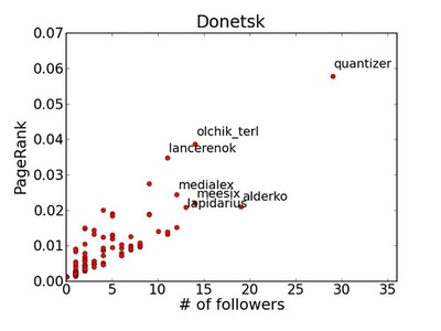
PageRank
Iterative eigenvector-style algorithm modeling a random surfer to rank nodes by importance. Converges over iterations; damping and teleportation stabilize results. Widely used for ranking and centrality.
Spectral clustering
Uses eigenvectors of the graph Laplacian to embed nodes, then clusters in that space. Effective for non‑convex cluster shapes; computational cost dominated by eigen decomposition on large graphs.
Louvain method
Greedy, hierarchical optimization of modularity that aggregates nodes into communities and repeats. Extremely fast and scalable in practice; finds high-modularity partitions but can be sensitive to resolution.
Girvan–Newman
Removes edges with highest betweenness to split communities iteratively. Intuitive and useful for small networks or analysis, but computationally heavy for large graphs.
Label propagation
Nodes adopt the most frequent label among neighbors iteratively until convergence. Simple, near-linear, and scalable, but nondeterministic and may produce varying results.
Node2vec
Generates biased random walks to capture network homophily and structural roles, then trains skip-gram to produce node vectors. Flexible parameters balance breadth-first and depth-first exploration.
DeepWalk
Performs uniform random walks from nodes and learns representations via language-model techniques. Simple and effective for many tasks; precursor to node2vec with fewer hyperparameters.
LINE
Optimizes objectives to preserve local (first-order) and neighborhood (second-order) proximities, designed for very large graphs with efficient stochastic training.
Weisfeiler–Lehman test
Iterative color-refinement procedure distinguishing many nonisomorphic graphs; used as a fast test and as a feature extractor in graph kernels and ML pipelines.
K‑core decomposition
Iteratively removes vertices with degree < k to reveal nested cores, highlighting densely connected subsets. Fast and useful for identifying influential or cohesive groups in networks.
Chinese Postman (Route inspection)
Finds minimum-length tour covering all edges by pairing odd-degree vertices and adding matching edges. Exact solution for route inspection problems on undirected graphs.
Christofides’ algorithm
Constructs MST, matches odd vertices, and shortcuts to produce a tour with provable 1.5 approximation for metric TSP. Practical when exact TSP is infeasible and metric properties hold.
VF2
Backtracking algorithm for subgraph and graph isomorphism with pruning rules that perform well in practice. Used in cheminformatics and graph query engines; worst-case exponential but efficient on many inputs.
Karp’s minimum mean cycle
Finds cycles minimizing average weight per edge using dynamic programming. Useful for detecting negative cycles or optimizing repeating processes in weighted directed graphs.
Graph coloring (DSATUR)
DSATUR is a heuristic that selects vertices by saturation degree to color graphs with few colors quickly. Useful when exact coloring is infeasible; produces high-quality solutions in practice.
Subgraph centrality (spectral)
Spectral measure counting closed walks weighted by length using eigen decomposition. Highlights nodes involved in many small substructures; informative but computationally heavy for large graphs.
Maximum spanning forest
Variant of MST that selects maximum-weight edges to form a forest when graph is disconnected. Useful for building strongest-connectivity backbones or diversity-aware networks.
Minimum feedback edge set
Finds smallest set of edges whose removal makes a graph acyclic. Exact solutions are hard; approximations and heuristics are used in practice for dependency cleanup.
K‑means on graph embeddings
Not a graph-native algorithm but commonly applied to node embeddings to cluster nodes. Use after embedding methods (DeepWalk, node2vec) to produce partitions in vector space.