In 2012, AlexNet dramatically improved image-classification accuracy on the ImageNet dataset, showing that deep neural networks could outperform prior methods on complex perception tasks.
That success—ImageNet had roughly 1.2 million labeled images—made a practical point: deep neural networks scale in depth and parameters in ways classical algorithms do not. Understanding the differences between deep learning and machine learning matters for practitioners, managers, and students because picking the wrong approach wastes time, budget, and often trust in a project.
This article treats deep learning as a specialized subset of machine learning with distinct trade-offs across architecture, data, interpretability, compute, and deployment. Below are seven concrete differences grouped into three themes: Foundations & Architecture; Data & Training; and Performance, Deployment & Use-cases.
Foundations & Architecture
This group covers structural and conceptual contrasts: how models are built, how they represent data, and what milestones shaped current practice. Think of shallow models as a single-story house and deep models as a multi-floor tower—both shelter data, but they do so very differently.
1. Model complexity and architecture
Deep learning models typically contain many more layers and parameters than classical machine-learning models. Small convolutional networks already reach millions of parameters; large language models scale to billions (GPT-3 is a common reference at 175 billion parameters). ResNet (introduced in 2015) showed that very deep nets—ResNet-152 and similar—could be trained reliably using residual connections.
By contrast, logistic regression, small neural nets, or tree ensembles often contain far fewer effective parameters and much less depth. That lower complexity helps on structured, low-dimensional problems and when interpretability matters.
Architectural choices drive capability on unstructured inputs—images, audio, raw text—where hierarchical feature extraction and depth give clear advantages. But for small-tabular datasets, simpler models (logistic regression, random forests, XGBoost) remain preferable because they are faster to train, cheaper to run, and less prone to overfitting.
2. Feature engineering versus representation learning
Classical machine learning often relies on manual feature engineering: domain experts design SIFT or HOG descriptors for images, MFCCs for audio, or carefully normalized fields for tabular data. Those hand-crafted features inject human priors into models.
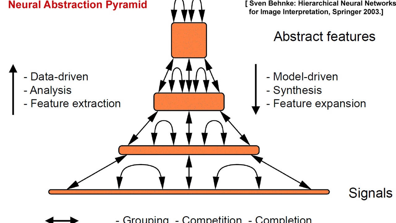
Deep learning flips that model: convolutional networks, recurrent nets, and transformers learn hierarchical representations directly from raw inputs. End-to-end systems like DeepSpeech demonstrated that models can learn useful audio representations from spectrograms without MFCCs, and ImageNet-pretrained CNNs provide feature maps that transfer to medical imaging or remote sensing.
The trade-off is practical. Classical pipelines spend time on feature design and domain rules; deep pipelines spend time collecting labels and computing. Transfer learning and pretraining (ImageNet, large-language-model pretraining) help reduce labeled-data needs by reusing learned features.
3. Interpretability and transparency
Deep models are generally less interpretable than many traditional models. A decision tree with depth under ten is human-readable; a CNN or transformer with millions of weights is not. That opacity matters in regulated industries like healthcare, insurance, and finance.
Tooling exists to help—LIME and SHAP provide local feature explanations, saliency maps highlight image regions, and attention visualizations help inspect transformer behavior—but these are imperfect and sometimes misleading. Post-hoc explanations rarely equal the clarity of an inherently transparent model.
Mitigations include choosing smaller interpretable models, using model distillation to create simpler surrogates, or constraining architectures to be more transparent. Where compliance or clinician trust is necessary, the added cost of interpretability often outweighs raw performance gains.
Data and Training Considerations
This section focuses on how data scale, labeling effort, and compute differentiate deep approaches from classical ones. Sample efficiency and resource demand often determine whether a project is feasible.
4. Data requirements and sample efficiency
Deep learning often requires much larger labeled datasets to reach top performance; ImageNet is a canonical example with approximately 1.2 million labeled images in mainstream experiments. Classical algorithms frequently do well with hundreds to a few thousand clean samples.
Fine-tuning a pretrained CNN can succeed with a few thousand labeled examples rather than millions—a practical route used when data collection is costly. Techniques like data augmentation, synthetic labeling, and few-shot learning further improve sample efficiency.
Labeling cost matters. Simple crowdsourced labels might run $0.10 per image, while expert annotations (radiology reads, legal review) can cost $50–$500 per sample. For many teams, labeling and annotation budgets dominate model selection decisions.
5. Training cost and compute
Training deep models usually requires significant compute. Large transformer training jobs can take hundreds to thousands of GPU-hours; models at the GPT-3 scale took weeks on hundreds of GPUs or TPUs and incurred multi-million-dollar bills to train in the cloud.
By contrast, many classical methods train quickly on CPUs—in minutes to hours—even on modest machines. Secondary costs matter too: energy consumption, cluster management, and storage of large checkpoints all add to project budgets.
Teams control costs with strategies like mixed-precision training, pruning and distillation, transfer learning from pretrained checkpoints, or selecting smaller architectures such as MobileNet for constrained environments. Those tactics can cut compute needs by an order of magnitude in some cases.
Performance, Deployment, and Use Cases
Here we compare where each approach shines in production, and what operational trade-offs to expect. Consider both technical fit and lifecycle costs when choosing a path.
6. Performance ceilings and task suitability
Deep learning tends to outperform when inputs are high-dimensional and unstructured—images, raw audio, and free-form text. Benchmarks like ImageNet (vision) and GLUE (NLP) show clear transformer and CNN dominance in those domains.
However, classical machine-learning techniques frequently match or beat deep nets on structured, tabular problems. XGBoost and similar tree ensembles still dominate many Kaggle tabular leaderboards because they encode useful inductive biases for those feature types.
A pragmatic rule: run quick baselines with logistic regression, random forests, or XGBoost before committing to deep architectures. That step reduces risk and often identifies whether the extra complexity of deep models is justified for the task.
For readers weighing the differences between deep learning and machine learning, start by classifying your data (structured vs unstructured), your sample size, and the expected accuracy gains from richer models.
7. Deployment complexity and maintenance
Deploying deep models usually involves more engineering. Modern CNNs can be tens to hundreds of megabytes; large language models can be many gigabytes. Inference latency, memory footprint, and accelerator dependence (GPUs/NPUs) matter for real-time systems.
Operational tasks include versioning large artifacts, monitoring model drift, and scheduling continuous retraining when data distributions shift. These add people and tooling costs compared with deploying a small scikit-learn model that fits in a few megabytes and serves on a CPU.
Tools and optimizations help. Model pruning, quantization, and distillation reduce size and latency. Frameworks like TensorFlow Lite and ONNX Runtime support edge and cross-framework deployment; MobileNet offers architecture choices designed for mobile inference. MLOps platforms simplify CI/CD for models, but they do add platform costs and operational overhead.
Summary
- Match model choice to the problem: deep architectures shine on unstructured, high-dimensional data; classical algorithms remain strong for tabular and small-sample tasks.
- Consider data and compute first—ImageNet (~1.2M images), GPT-3 (175B parameters) and multi-week GPU runs are useful benchmarks to estimate effort and cost before scaling up.
- Prioritize a quick classical baseline (logistic regression, random forest, XGBoost), measure labeling and infrastructure costs, then escalate to deep models if the expected gains justify them.
- Factor in interpretability, latency, and operational complexity when deciding between deep learning and machine learning—regulatory needs or tight latency budgets often favor simpler models or optimized deep variants.
- Checklist: data size, compute budget, interpretability requirements, and latency targets. Follow that order when planning experiments and procurement.