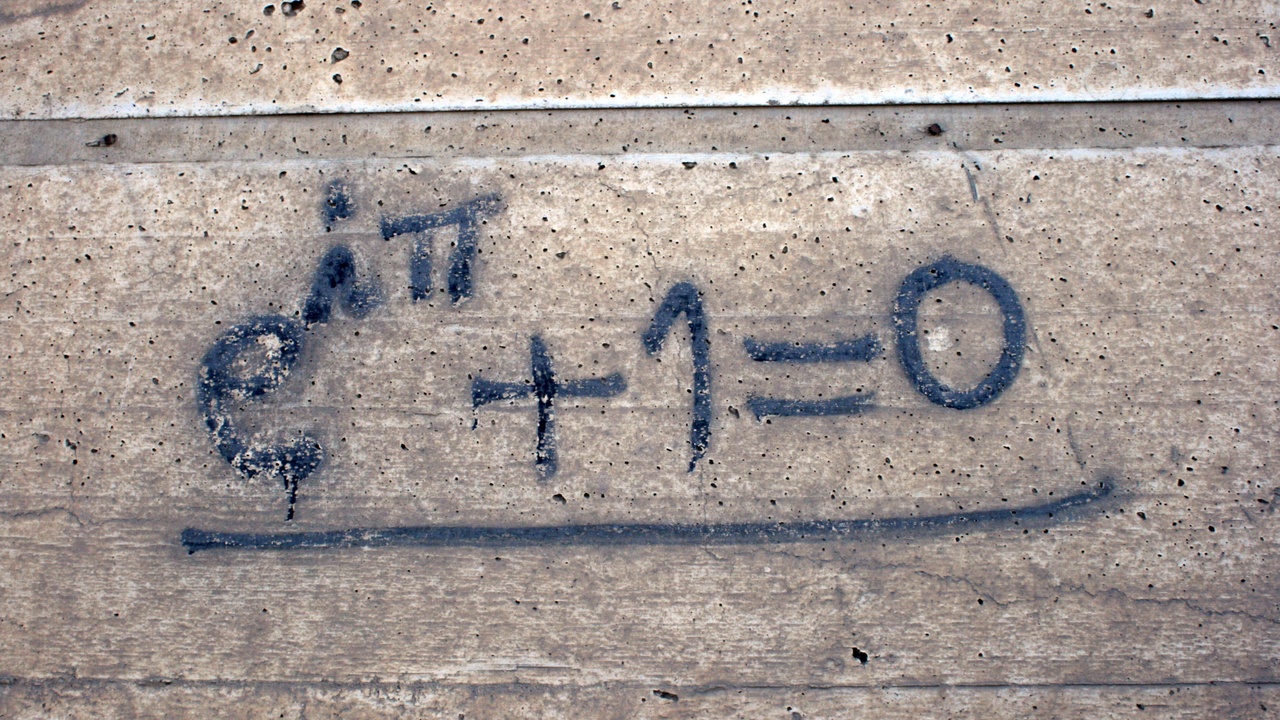
Euler’s 1748 formulation e^{ix} = cos x + i sin x tied sine and cosine to complex analysis and made their relationship both deep and concrete.
So why bother with the fine-grained differences between sine and cosine? Students, engineers, and data practitioners all run into cases—root finding, Fourier modeling, or phased signals—where knowing which function to use (and why) changes outcomes.
This piece lays out seven clear differences between sine and cosine, grouped into three categories: mathematical properties, graphical and calculus differences, and application/computation contrasts. Expect concrete formulas, short examples (π, π/2, 2π appear often), and practical notes you can test in MATLAB or NumPy.
Mathematical Foundations
Although sine and cosine are phase-shifted cousins and connected by derivatives, three formal differences in definitions, periodic placement of zeros and extrema, and parity drive much of their distinct behavior.
1. Definitions and fundamental identities
On the unit circle at angle θ the coordinate pair is (cos θ, sin θ): cosine is the x-coordinate and sine the y-coordinate. Euler put this relation into a compact complex form in 1748 with e^{iθ} = cos θ + i sin θ, which explains many algebraic identities.
Key identities include sin^2 x + cos^2 x = 1 and the angle-sum formulas:
sin(x + y) = sin x cos y + cos x sin y, and cos(x + y) = cos x cos y − sin x sin y.
Concrete values at common angles: sin 0 = 0 and cos 0 = 1; sin(π/6) = 1/2 and cos(π/6) = √3/2; sin(π/2) = 1 and cos(π/2) = 0. These starting values feed into series, boundary conditions, and small-angle approximations used later.
2. Domain, range, and periodic behavior
Both functions are defined for all real x, take values in [−1, 1], and repeat every 2π: f(x + 2π) = f(x). Yet the locations of zeros and extrema differ by π/2.
Sine has zeros at x = nπ (… , −2π, −π, 0, π, 2π). Cosine has zeros at x = π/2 + nπ (…, −3π/2, −π/2, π/2, 3π/2). Sine attains maxima at x = π/2 + 2πn; cosine attains maxima at x = 2πn.
That shift matters practically: zeros set boundary conditions in ODEs (for example, solving y” + y = 0 with y(0)=0 leads naturally to sine solutions), and the distinct extrema locations guide sampling in signal acquisition.
3. Symmetry and parity: odd vs even
Sine is odd: sin(−x) = −sin x. Cosine is even: cos(−x) = cos x. That simple algebraic sign difference has concrete consequences.
Because of parity, Fourier series separate cleanly: an odd function’s Fourier expansion contains only sine terms, while an even function’s expansion uses only cosine terms. Integrals simplify too: ∫_{−a}^{a} sin x dx = 0 by oddness. For cosine, ∫_{−π}^{π} cos x dx = 0 as well, but because the interval covers a full period (2π) and the positive and negative lobes cancel over that span.
Parity affects PDEs and modal decompositions: choosing sine or cosine basis functions changes which boundary conditions (Dirichlet vs Neumann) are satisfied automatically.
Graphical and Calculus Differences
Graphs, phase, slopes, and curvature expose how a mere shift and a sign change in derivatives create distinct practical behavior. Two items are especially useful: the π/2 phase relation and the derivative pairing.
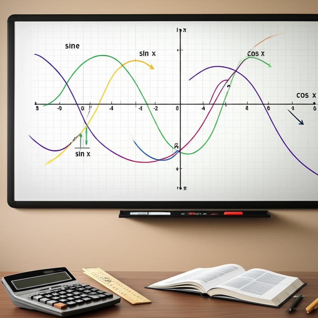
4. Phase shift and graph alignment
The fundamental phase relation is cos x = sin(x + π/2) (equivalently sin x = cos(x − π/2)). A π/2 (90°) shift moves peaks into zero crossings and vice versa.
Compare values at a few angles: at x = 0, sin 0 = 0 while cos 0 = 1. At x = π/4, sin(π/4) = √2/2 and cos(π/4) = √2/2 (they match there). At x = π/2, sin(π/2) = 1 while cos(π/2) = 0. That shift is why two otherwise identical oscillators can be said to be in quadrature when they differ by 90°—a central idea in I/Q modulation and quadrature demodulation used in Wi‑Fi and software-defined radio.
5. Derivatives, integrals, and differential behavior
The derivative pair is compact: d/dx[sin x] = cos x and d/dx[cos x] = −sin x. Differentiation therefore effects both a phase shift and, for cosine, a sign inversion.
At x = 0 the numerical slopes reflect that: sin'(0) = cos 0 = 1, while cos'(0) = −sin 0 = 0. For second derivatives, sin” = −sin and cos” = −cos, which is why solutions to y” + y = 0 are linear combinations of sin and cos with initial conditions selecting the particular combination.
Taylor series near zero make the starting-value difference explicit: sin x = x − x^3/3! + x^5/5! − …, while cos x = 1 − x^2/2! + x^4/4! − …. The sine series starts at 0 (no constant term) and the cosine series starts at 1, so small-angle approximations (sin x ≈ x, cos x ≈ 1 − x^2/2) behave differently for tiny x.
Applications, Computation, and Practical Differences
When you move from pen-and-paper math to code and hardware, the choice between sine and cosine matters for representation, compression, and numerical robustness.
6. Representation in Fourier series and transforms
Even and odd parts of a signal determine whether cosine or sine terms appear in a Fourier series. An even signal has cosine-only coefficients; an odd signal has sine-only coefficients. That simplifies computation and interpretation.
Consider a square wave centered at zero: its Fourier series contains only odd sine harmonics with amplitudes proportional to 1/n. The Discrete Cosine Transform (DCT), by contrast, uses only cosine basis functions—this choice reduces boundary discontinuities and is why JPEG and many MPEG profiles use an 8×8 DCT block for image compression.
For smooth signals the Fourier coefficients decay quickly, so knowing whether sine or cosine terms dominate helps predict convergence and compression performance.
7. Computational choices and engineering practicalities
In numerical work the two functions differ in starting values and in how implementations handle extreme arguments and round-off. For tiny angles (say |x| < 0.1 rad) the approximation sin x ≈ x gives a cheap, accurate shortcut; cos x ≈ 1 − x^2/2 is the corresponding small-angle form.
Practical tips: call library routines (NumPy’s np.sin, np.cos or math.h in C) for stability rather than writing your own polynomial unless performance demands it. Many FFT libraries (FFTW, Intel MKL) use hardware trig or lookup tables for speed.
Embedded examples: when implementing an oscillator on a microcontroller it’s common to store cos(θ) as a phase reference and generate the quadrature partner via sin(θ) = cos(θ − π/2). On test equipment, an oscilloscope will show a 90° phase shift between current and voltage for a purely inductive or capacitive load—practical evidence of the geometric π/2 relation.
Summary
- Parity and starting values matter: sine is odd and starts at 0; cosine is even and starts at 1, which affects Fourier expansions and small-angle approximations.
- The single geometric fact—a phase shift of π/2—explains many graphical and signal-processing differences, including quadrature in I/Q systems.
- Derivatives and Taylor series differ in sign and initial terms (sin x = x − x^3/3! + …; cos x = 1 − x^2/2! + …), which changes ODE initial-condition behavior and numerical approximations.
- In practice, choose bases and implementations deliberately: cosine bases (DCT) are standard in JPEG; sine-only or cosine-only Fourier series simplify coefficient computation; use library trig functions (NumPy, FFTW, math.h) and verify phase when combining signals with an oscilloscope or in embedded code.